5. Entanglement, Partial Traces and Bloch Vectors
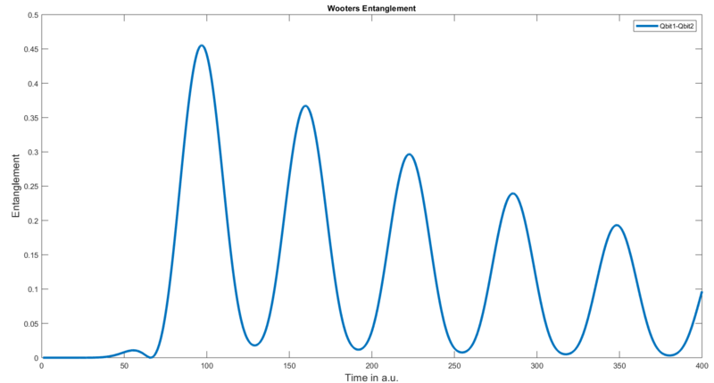
This chapter delves into some advanced functions that are useful in the context of quantum computing. The entanglement between two qbits is vital for quantum computing operations yet, surprisingly bad defined. There exist several measurements for entanglement. A very popular one is the so called concurrence. Unfortunately, this measurement is only valid for pure states (states that have undergone no decoherence process), for arbitrary two qbit states, Wootters measure for entanglement is more suitable (see [1]). It is quite complex to calculate, but fortunately, the Toolbox provides a getEntanglement(name1,name2) method that returns Wootters entanglement between the two qbits with name1 and name2. See the following example:
1 | s = System; %create a System |
By now the code should look fairly familiar. We have a system of two coupled qbits. getEntanglement does not need any parameters since it can only work on a density matrix of two qbits. The resulting plot looks like this:
But now suppose we have more than two qbits in our simulation, like in the cavity example. The entanglement between them still carries physical meaning but the density matrix is much larger and we cannot extract the entanglement directly.
This is where partial traces come in. Partial traces (which have (almost) nothing in common with the typical trace of a matrix) allow us to “filter out” a specific subsystem. The resulting density matrix is of lower dimensions and describes all subsystems that have not been traced out. This can generally be useful for many applications. In this tutorial, we will only use it for entanglement. The traceOut(name) method of the system class has to be called after a finished simulation. The reduced density matrices will be available in another three-dimensional array called "reduced_rho_hist". Multiple subsystems can be traced out sequentially. The getEntanglement method works on the reduced density matrices if they have the right dimensionality and otherwise throws an error. Take a look at this example:
1 | s = System; %create a System |
The code above yields the following figure:
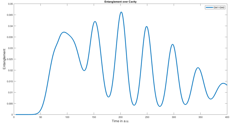
As a next step you could, for example, add energy or population plots to this figure and see how to entanglement behaves in relation to these.
Bloch vectors are a tool to examine the state of a qbit in more detail. The System class provides the methods blochsphere(name) and animateBlochsphere(name). To learn about their function, please take a look at the Matlab documentation.