3. Specific coupling, Dissipation, and Dipoles

Up to this point, we have been working with qbits, and for a qbit, the mechanisms for coupling, dissipation and external laser pulses that have been presented so far are sufficient. However, suppose we have a system that consists of two three-level subsystems A and B. Now, the transition between states |0> and |1> of subsystem A can couple to the |0> – |1> transition of subsystem B with a different strength than, for example, the |0> – |2> transition of A to the |1> – |2> transition of B. In other words, we need a way to set, enable and disable the coupling between arbitrary level transitions. To do this, no additional command is necessary. Rather the addCoupling method is heavily overloaded. Take a look at the following code:

This implements a system in which only the |0> – |1> transitions of A and B couple to each other. We can take a look at the resulting diagonal elements of the density matrix using the plotoccupation command of the System class  (the plotoccupation command always plots all diagonal elements of the density over time, if you do not specify parameters).

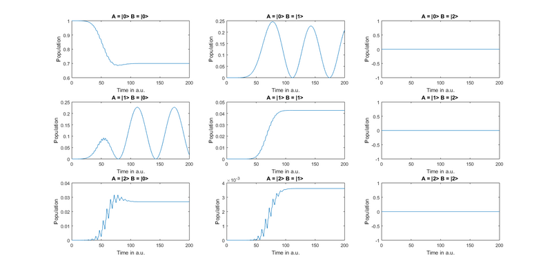
As you can see, the laser shifts substantial population in the A= |2> B = |0> state. However, this population never decreases, since there is no coupling term which couples it to the A = |0> B = |2> state.  The "[1 0]" behind the "A" in the addCoupling command defines that this coupling is only valid for the |0> – |1> transition in subsystem A. The same goes for the [1 0] term behind "B". If we leave out such a term, the coupling is implemented for all transitions of a subsystem. So if the [1 0] behind "B" were missing, the |0> – |1> transition of A would couple to all transitions of subsystem B. And if both "[1 0]" were missing, all transitions of A would couple to all transitions of B. So if you want different coupling strengths between different transitions, you can use multiple specific addCoupling commands. Note that addCoupling adds a dipole–dipole Hamiltonian to the system that is inherently resonant dependent. Thus, even if a transition of energy E = 1 a.u. has a strong coupling strength to a transition of E = 1.5 a.u., almost no energy will be transferred (unless you have a very large line width due to dissipation and dephasing).

The same principle applies to dissipation and dephasing terms. Population decays with different rates between |1> – |0>, |2> – |0> and |2> – |1>. In order to add a specific dissipation between |1>  and |0> of subsystem A to the simulation, use:

Again, if the third parameter is not supplied, addDissipation will add a dissipation effect between all possible level transitions.

The toolbox is structured as such that if you are just starting and have not yet invested any thought on advanced topics, you can still use it. If, after a bit of tinkering, you find that “I am missing this and that … “, you can usually add it easily by supplying additional parameters to the same commands you have used before.

Lastly, we have external laser pulses. These will interact with a transition in a subsystem according to the dipole moment of that transition. Consequently, we need a way to set dipole moments. (At the present, the toolbox only supports scalar dipole moments and scalar electric fields. If you have a molecule in which different dipole moments stand at different angles to the incoming field, you will have to capture that by setting the dipole strength.) The Nlevel class has the necessary method which is fittingly called setDipole. To use the setDipole method, the Nlevel object has to be defined separately and later added to the overall system:

As the first parameter, setDipole takes the levels between which the dipole moment is set. The second parameter is the dipole moment. By default, all dipole moments are set to one (again in atomic units).

Note: If the setDipole commands is called once, all other dipole moments of the subsystem are set to zero! If one dipole is manually defined, all dipole moments must be user supplied.

Defining a subsystem separately has the additional benefit of the user being able to look at all the variables of the created object, for example the dipole matrix, by using the standard Matlab interface.