2. Dissipation, Dephasing and Laser Pulses
In order to increase the realism of our simulation we are missing two main ingredients that are present in almost every experimental setup. External laser pulses that excite the system and the dissipation and dephasing a quantum system undergoes as it interacts with the environment.
Dissipation and dephasing are implemented via the Lindblad formalism (for more detailed information take a look at the documentation of the addDissipation function or the paper). In order to add a dissipative channel to qbit1 we add the following line of code to the above source code (at any place after qbit1 has been defined and before the simulation command is called):
s.addDissipation('qbit1',50);
This command results in the following figure:
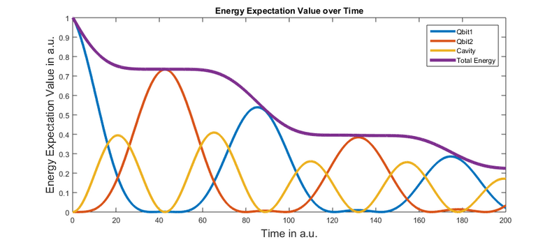
As parameters the addDissipation function takes the name of the subsystem that is losing energy to the environment and the lifetime of the excited-state population. Consequently, after 50 a.u., the excited state population of qbit1 decays to 1/e-th of its original value. Note that the population is only decaying if there is actually population in qbit1. We have added the overall energy expectation value of the system to the plot. As you can see, the energy expectation value is only declining if there is energy (and thus excited-state population) in qbit1.
The dephasing command works analogously and allows the user to implement a pure dephasing process that results in loss of phase information within the system but no loss of energy.
Arbitrary external fields can be added via the addExternalField command which takes two parameters: an external field function and the subsystem the external field interacts with. Lets take a look at how this looks in practice:
1 | clear; close all; |
That looks really complicated. What is Gausspulse and why does it have that many parameters? Don’t worry, Gausspulse is actually something you can define yourself. Here is the Matlab function, which is also a template you can use for any field function you want to define:
1 | function [ out ] = Gausspulse(amp,td,tp,we) %td = delay time, tp = pulse width, we = frequency |
The outer function returns a pointer to the inner function (which is named appropriately). The idea behind this is that the inner function, which is passed to the System object, always needs a single parameter which is the time vector. The time vector is then later supplied by the System class. The structure is build in this way, since the System object cannot have knowledge of any other variables of your laser-pulse function like the pulse duration. Thus, the outer function takes all those other parameters. In the case of Gausspulse these are: amplitude, time delay, pulse duration and frequency. This is how the above defined laser pulse looks like:
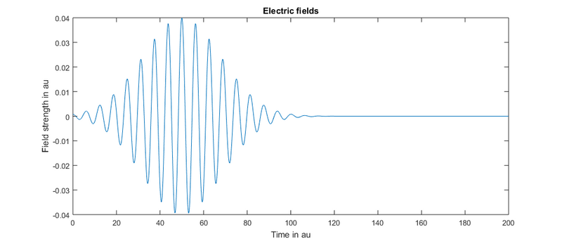
You can generate this plot easily by using the plotEfields function of the system class. If we execute the latest iteration of our simulation and plot the energy values, we get:
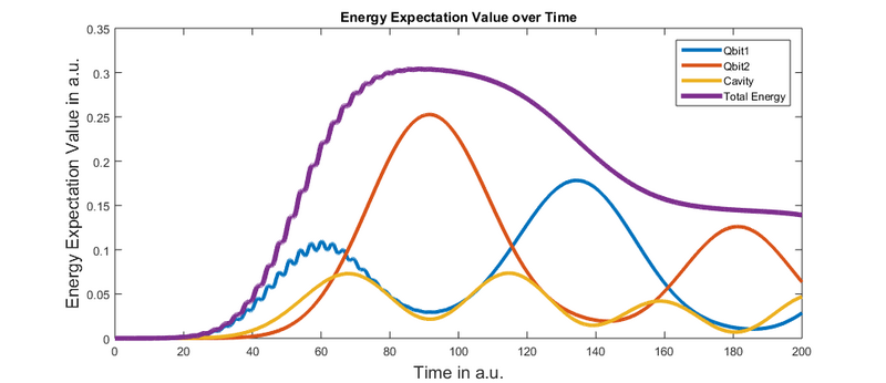
Note that we removed the line in which we set qbit1 in an excited state at the start of the simulation and we also added a line for a dissipative channel of qibt1. As you can see, the system starts with all entities in the basic state and at first absolutely nothing happens. As the laser pulse acts on the system, energy is transferred into qbit1 and subsequently transferred into the cavity and qbit2. Interestingly, the highest amplitude in energy expectation value and thus population at any time is held by qbit2, which does not directly interact with the external field.