4. Polarization, Fourier Analysis und Susceptiblity

Another variable of interest is the polarization of a subsystem, since it is often accessible via an experiment. QDT provides a getPolarisation(name) function which returns the polarization over time of a certain subsystem. The polarization operator is dependent on the different dipole moments between levels, which can be set by the setDipole method. The getPolarisation method takes these dipoles into account.

1 2 3 4 5 6 7 8 9 10 11 12 13 14

s = System; %create a System s.addEntity(Nlevel(1),'qbit1'); %add the created qbit and call it qbit1 s.addEntity(Qoscillator(3,1),'cavity'); %add a quantum harmonic oscillator with 5 levels and energydiffernce of 1 a.u. s.addCoupling('qbit1','cavity',0.05); %add a coupling between the first qbit and the cavity s.addDissipation('qbit1',50); %Set the lifetime of qbit1 to 50 a.u. s.addDissipation('cavity',50); %Set the lifetime of the cavity to 50 a.u. s.addExternalField(Gausspulse(0.04,50,30,1),'qbit1'); %set an external electric field that interacts only with qbit1 %done s.setTmax(400); %set the maximum time s.setTimestep(0.1); s.simulate; % start the simulation h = plot(s.time,s.getPolarisation('qbit1'));

The above example plots the polarisation of one qbit in a cavity and results in the following figure:

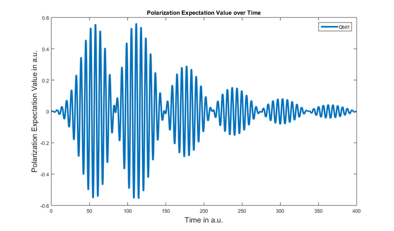
However, it is quite difficult to interpret this data. To gain more information, we need to perform a Fourier analysis.

The standard FFT (Fast Fourier Transformation) implementation returns a mirrored spectrum and does not provide the associated frequency array which is prone to error. For this reason, the System class provides its own fft function and supplies the fitting frequency array. Furthermore, the setdf method is provided. If this method is invoked, the frequency array is newly constructed with the new frequency increment. Moreover, all future calls to the System object’s fft method will trail the input data with zeros to achieve the necessary signal length. Performing

plot(2*pi*s.f, abs(s.fft(s.getPolarisation(‘qbit1′))),’o’); axis([0 2 -inf inf]);

results in:

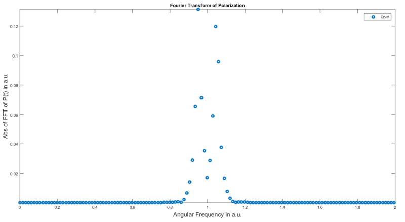
which is not bad, but the resolution is a little too low for our liking.  Note the parameters of the above plot command. "s.f" contains the frequency array that is managed by the System class. "s.fft" performs a Fourier transform on the provided array (this array must have the same length as the System class time array; all System functions like getEnergy will return such an array). Since the resulting array is complex, we take the absolute value of its entries using Matlab’s "abs" function.

In order to increase the resolution of our Fourier-transformed signal we can use the setdf function. Calling

s.setdf(0.0001); h =plot(2*pi*s.f, abs(s.fft(s.getPolarisation(‘qbit1′))),’o’); axis([0 2 -inf inf]);

results in:

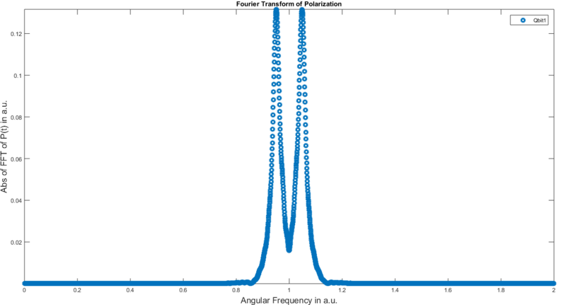
We can now clearly see the two relevant peaks which are centered around the resonance frequency. There are two peaks instead of one, since the qbit and cavity couple with each other, and thus, analogously to two classical pendulums, one mode with a higher and one with a lower resonance frequency are created. Depending on the coupling strength, this effect is stronger or weaker.

Susceptibility

The susceptibility can be viewed of as a measure of the systems reaction, normalized by the applied external field. To calculate it, QDT provides the getSusceptibility function. For more information see the Matlab documentation.